What is ordinal utility?
Ordinal utility depicts the customer’s satisfaction level by viewing his preferences of one product over the others. The ordinal utility theory explains that it is meaningless to ask how much better one good is as compared to another. Therefore, all these studies of customer decision making are expressed in terms of ordinal utility. Pareto introduced the concept of ordinal utility.
For example, if Advait prefers A over B and B over C which can also be explained with numbers. Then the theory of ordinal utility finds numeric representation as meaningless. However, the ordinal utility also focuses on the difference of preferences as well among the products by the consumer.

Conditions for existence of ordinal utility
- Transitivity: It explains the relation if A > B and B > C then A > C. Therefore, if a customer chooses A over B and B over C then he must choose A over C according to the order of preferences determined by transititvity.
- Completeness: If A, B are subset of X, then either A < B or B < A or both
- Continuity: The concept of continuity depicts that if A is preferred over B then even small deviations from both will not lead to reversing their order.
- Uniqueness: For all utility function, there is an ideal and unique relation while the opposite might not be true. A preference relation can be depicted by various utility functions. However, the same preferences of the customer can be represented by any ordinal utility function with monotonically increasing transformation.
- Monotonicity: Like if a preference relation is monotonically increasing explains more is always better (where the ordinal utility is positive).
Measures of Economic Utility
There are specifically two measures of economic utility definition namely ordinal utility and cardinal utility which is discussed under :
Cardinal Utility
According to the cardinal utility, the utility of a commodity can be measured due to which it can be added, subtracted, or compared. It denotes/measures the utility in terms of utils. Like if an apple provides 10 utils of utility and a banana provides 20 utils, so it can be said that a banana has double satisfaction ability than an apple.
Ordinal utility
Whereas the ordinal numbers stand 1st, 2nd or third etc till so on. This explains the customer’s order preference of the product or its choice but it does not describe how much he prefers one to the other.
The marshall utility is based on cardinal prospect while the Hicks follows the psychological and subjective aspect of ordinal utility. As a result, Hicks rejects the quantitative aspect and measures ordinally the indifference curve technique.
Cardinal vs ordinal utility
Many theories focus on the level of satisfaction. However ordinal utility and cardinal utility are two major theories highlighted. The cardinal utility entrusts to measure the satisfaction in utils while ordinal utility determines it cannot be evaluated but levelled.
The below discussion further elaborates the point to support the differentiation of cardinal vs ordinal utility:
| Parameters | Cardinal utility | Ordinal utility |
| Definition | The cardinal utility represents the satisfaction level of goods or services in terms of numbers after their consumption. | The ordinal utility acts opposite of the cardinal saying it cannot be scaled in numbers. While they can be arranged in order of preferences. |
| Example | Sandwich gives 60 utils of satisfaction while pizza provides 30 utils to Advait. | Sandwich provides greater satisfaction to Advait than Pizza. |
| Measurement | Measured in utils. | The ordinal utility is ranked concerning satisfaction. |
| Realistic | Less practical | More practical and sensible |
| Used by | Applied by professor Marshall | Applied by Prof. J.R Hicks |
| Consumer equilibrium names | Utility analysis | Indifference curve analysis |
Indifference curve
It shows different combinations of two goods that provide the same level of satisfaction to the customer. For example, a consumer is indifferent among the following consumption bundles A ( 1,10 ), B ( 2,6 ), and C ( 3,3 ). Hence, all these consumption bundles will lie on the same indifference curve i.e gives the same level of satisfaction.
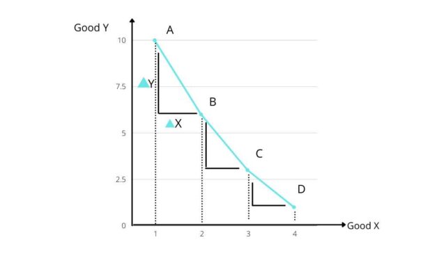
Properties of indifference curve
An indifference curve is downward sloping from left to right
This is because if a consumer is simultaneously consuming two commodities, he can increase consumption of one good in such a manner that total ordinal utility meaning remains unchanged/ constant. This is due to the monotonic preferences of the consumer.
According to monotonicity, a consumer prefers more of at least one good with no less of the other or more of both the goods. Hence, to lie on the same indifference curve, a consumer must decrease consumption of other goods to increase consumption of given goods. This makes the indifference curve downward sloping.
The indifference curve is convex to the origin
This is due to the diminishing marginal rate of substitution. MRS is the amount of good Y that a consumer is willing to sacrifice to increase the consumption of good X by one unit leaving total ordinal utility meaning unchanged. As consumption of X increases, the marginal utility of X decreases. Hence, a consumer is willing to sacrifice lesser and lesser of Y. In other words, MRS decreases.
Indifference curve lying to the Right represents a higher satisfaction
Any consumption bundle on a higher indifference curve represents either more of both the goods or more of both the goods or more of at least one good with no less of the other.
Indifference curve analysis is based on assumption that preferences are monotonic which means more consumption gives more satisfaction. Hence, a higher indifference curve represents higher satisfaction.
Two indifference curves cannot intersect each other
Suppose two indifference curves intersect each other at point B, then we get a contradictory result in terms of preference writing. In the diagram, the consumer is indifferent between A and B opting for both.
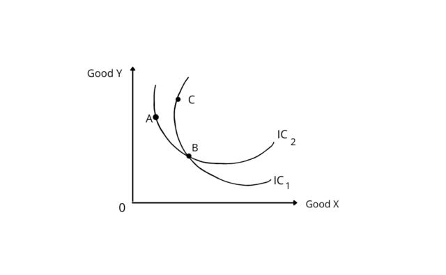
According, to the property of transitivity, the consumer will be indifferent between consumption bundles A and B but it is clear that C is preferred over A as it has more of both goods. Therefore, a contradiction appears.
Marginal Rate of Substitution
- The marginal rate of substitution is defined as the amount of good Y that a consumer is willing to sacrifice to increase consumption of good X by 1 unit leaving total ordinal utility meaning unchanged.
- Graphically, MRS is the slope of the indifference curve,
MRS = Change in Y / Change in X = Y2 – Y1 / X2 – X1
( negative sign indicates downslope)
- The marginal rate of substitution is diminishing i.e as consumption of X increases, consumers willingness to pay for good X in terms of good Y decreases. This is because, with the increase in consumption of X, MUx decreases. (since additional satisfaction obtained from X decreases)
- Hence, the consumer is willing to sacrifice a lesser and lesser amount of good Y i.e MRS decreases. Diminishing MRS gives rise to the convex shape of the indifference curve. (relating to the concept of consumer equilibrium meaning)
Note: Now, the character of diminishing marginal rate of substitution can be explained briefly (related to mrts in economics). As the consumer increases the consumption of X, the marginal utility of the X decreases. However, due to the sacrifice of Y its marginal utility increases.
According to the given equation above, MRS decreases since the numerator or MU(x) decreases, and the denominator increases. Hence the diminishing marginal rate of substitution arises due to the convex shape of the indifference curve or the reduction in the willingness to sacrifice Y to increase one unit of X.
Marginal rate of substitution in different preferences
- Firstly, in the case of perfect substitutes, the indifference curve is linear whereas MRS = constant. The consumer is indifferent between both the commodities and gives him the same level of satisfaction (ordinal utility approach).
- Secondly, in the case of perfect complements, the indifference curve is L-shaped where MRS = 0 or infinity. Here the consumer wants both goods equally with each other together.
- Thirdly, the indifference curve has a typical convex shape by COBB-Douglas where the diminishing marginal rate of substitution prevails. Moreover, the consumer chooses the combination which gives the maximum level of satisfaction (ordinal utility approach).
Budget line
A budget line shows the different possible combinations of two goods X and Y that can be purchased by a consumer. When he spreads his entire income given the market price of the commodity.
Equation of a budget line:
Px.X + Py.Y = M OR Y =( – Px / Py) . X + M/ Py
The slope of the budget line: – Px / Py (ratio of prices or market rate of exchange MRE)
A negative sign indicates that the budget line is downward sloping
- The absolute value of slope measuring rate at which consumer can substitute good X for good Y when he is spending his entire income. It is the ratio of the number of units of good Y required to be sacrificed to obtain one more unit of good X.
- The slope of the budget line is Px / Py since Px and Py is constant. Therefore, the slope will also be constant. Hence, the budget line will be straight. It is downward sloping because to increase consumption of one good consumer has to decrease consumption of another good when he is spending his entire income.
Consumer equilibrium indifference curve /ordinal utility analysis
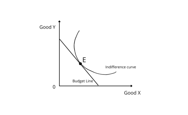
Conditions for consumer equilibrium indifference curve /ordinal utility analysis are:
- The slope of indifference curve = Slope of budget line OR
MRS = Px / Py OR MRS = MRE
- The marginal rate of substitution should be diminishing i.e indifference curve should be convex to the origin.
Note: MRS is defined as the amount of good Y that a consumer is willing to sacrifice (ordinal utility approach) to increase consumption of good X by 1 unit leaving total ordinal utility theory unchanged. While the ratio of prices is defined as the amount of good Y that a consumer is required to sacrifice to obtain/ increase consumption of X by 1 unit.
Explanation
- Initially, when a consumer starts consumption, MRS is greater than Px/ Py i.e to obtain one more unit of X a consumer is willing to sacrifice more than what he is required to sacrifice. Hence, the consumer gains and increases consumption of X. as a result, MUx decreases.
- Therefore, a consumer is willing to sacrifice less and less of Y each time he obtains one more unit of good X. As a result, MRS decreases and ultimately becomes equal to Px / Py at some combination of X and Y. At this combination, the consumer equilibrium is achieved.
- If the consumer intends to consume more X beyond consumer equilibrium, MRS will be less than Px/ Py i.e to obtain one more unit of X a consumer is willing to sacrifice less than what he is required to sacrifice.
- Hence, the consumer loses and decreases consumption of X. As a result, MUx increases. Therefore, the consumer is willing to sacrifice more and more of Y each time he obtains one more unit of good X. MRS increases and ultimately becomes equal to Px/Py at some combination of X and Y. At this combination, the consumer equilibrium is attained.
Conclusion
Therefore, ordinal utility emphasis the stress on the level of satisfaction without considering the numeric presentation and focus on the ranking system which is considered more reliable.
For a further explanation, we have an indifference curve that depicts the combinations of commodities chosen where the consumer is being indifferent providing the same level of the ordinal utility function. However, when studied with income of income or budget line, the consumer equilibrium can be known.